Comparison of multimodal GRNs

gretapy provides utilities to ease the comparison between multimodal GRNs, which contain TFs, CREs and target genes.

Here we will:

1. See available processed multiome datasets and download one

2. Run several method on them to get some GRNs to compare

3. Compare obtained GRNs at size, similarity and look for particular examples

Loading packages

import gretapy as gt
import scanpy as sc
import decoupler as dc

sc.set_figure_params(figsize=(3.5, 3.5), frameon=False)

Loading The Dataset

gretapy provides several already processed annotated multiome datasets. Here is to current list, which contains the name, the PUBMED ID of the original publication and the GEO ID where the data was retrieved if available:

datasets = gt.show_datasets()
datasets

	organism	name	pubmed	geo
0	hg38	Brain	38491288	GSE193688
1	hg38	Breast	39122969	None
2	hg38	Embryo	37369347	GSE218314
3	hg38	Eye	36277849	GSE196235
4	hg38	Heart	37438528	None
5	hg38	Kidney	37333123	None
6	hg38	Lung	39266564	GSE241468
7	hg38	PBMC	None	None
8	hg38	Pituitary	35263594	GSE178454
9	hg38	Repr. Fibroblasts	37873116	GSE242419
10	hg38	Skin	36121124	GSE207335
11	mm10	Palate	38280850	GSE218576

This is how to download one dataset, for example the Skin dataset:

Note

Any data gretapy downloads, it will be available at ./gretapy_data

breast = gt.ds.read_dts(organism='hg38', dts_name='Breast')
breast

MuData object with n_obs × n_vars = 3178 × 81920
  obs:	'batch', 'celltype'
  uns:	'neighbors', 'umap'
  obsm:	'X_spectral', 'X_umap'
  2 modalities
    rna:	3178 x 16384
      layers:	'counts'
    atac:	3178 x 65536
      layers:	'counts'

The obtained mudata.MuData consist of log-normalized counts of genes and genomic regions for ~3k cells with measurements for ~15k genes and ~65k regions.

The cell metadata stored in mudata.MuData.obs can be inspected.

breast.obs

	batch	celltype
ID13_AAACCAACACTGGCCA	ID13	Epithelial
ID13_AAACCAACAGGCCTTG	ID13	Endothelial
ID13_AAACCAACATCACTTC	ID13	Epithelial
ID13_AAACCGAAGCATTATG	ID13	Endothelial
ID13_AAACCGCGTAGACAAA	ID13	Epithelial
...	...	...
ID14_TTTGGTAAGCTTACTT	ID14	Fibroblasts
ID14_TTTGTCTAGTGAAGTG	ID14	Fibroblasts
ID14_TTTGTGAAGCCGCAGT	ID14	Endothelial
ID14_TTTGTGGCAGTTATCG	ID14	Fibroblasts
ID14_TTTGTTGGTATTGCAG	ID14	Adipocytes

3178 rows × 2 columns

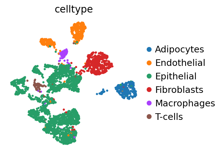
Cells can be visualized in UMAP space colored by cell type.

sc.pl.embedding(breast, basis='X_umap', color='celltype')

GRN inference

In this section we showcase how to perform GRN inference from a multiome dataset. We will run some of the baselines shown in the GRETA manuscript:

1. Literature derived networks: collectri and dorothea

2. Correlation based networks: pearson and spearman

3. A random network

Note

gretapy works with multimodal GRNs, meaning they should contain cis regulatory element (CRE) information in each edge. If your method is based on just transcriptomics data, you can transform it to multimodal by filtering interactions based on promoter accessibility, as it was done with all baselines in the GRETA manuscript.

You can easily achieve this by running:

# grn = pd.DataFrame with source and target columns, with optional weight column
mgrn = gt.mt.lit_grn(organism='hg38', grn=grn)

grn_dict = {}

# CollecTRI
grn_dict['CollecTRI'] = gt.mt.lit_grn(mdata=breast, organism='hg38', grn='CollecTRI')
grn_dict['CollecTRI'].head()

	source	cre	target	score
0	AHR	chr7-87600646-87601146	ABCB1	1.0
1	AHR	chr4-88230899-88231399	ABCG2	1.0
2	AHR	chr17-78186409-78186909	AFMID	1.0
3	AHR	chr7-16804717-16805217	AGR2	1.0
4	AHR	chr5-320864-321364	AHRR	1.0

# DoRothEA
grn_dict['DoRothEA'] = gt.mt.lit_grn(mdata=breast, organism='hg38', grn='DoRothEA')
grn_dict['DoRothEA'].head()

	source	cre	target	score
0	AHR	chr7-28298823-28299323	CREB5	1
1	AHR	chr5-138610325-138610825	CTNNA1	1
2	AHR	chr14-75278576-75279076	FOS	1
3	AHR	chr10-14329796-14330296	FRMD4A	1
4	AHR	chr5-66596058-66596558	MAST4	1

# Pearson
grn_dict['Pearson'] = gt.mt.correlation(mdata=breast, organism='hg38', method='pearson')
grn_dict['Pearson'].head()

	source	cre	target	score
0	PROX1	chr8-109362206-109362706	PKHD1L1	0.660204
1	MECOM	chr2-56183529-56184029	CCDC85A	0.648627
2	MECOM	chr13-28493920-28494420	FLT1	0.620280
3	MLXIPL	chr11-14642937-14643437	PDE3B	0.614183
4	MECOM	chr5-149141226-149141726	ABLIM3	0.611630

# Spearman
grn_dict['Spearman'] = gt.mt.correlation(mdata=breast, organism='hg38', method='pearson')
grn_dict['Spearman'].head()

	source	cre	target	score
0	PROX1	chr8-109362206-109362706	PKHD1L1	0.660204
1	MECOM	chr2-56183529-56184029	CCDC85A	0.648627
2	MECOM	chr13-28493920-28494420	FLT1	0.620280
3	MLXIPL	chr11-14642937-14643437	PDE3B	0.614183
4	MECOM	chr5-149141226-149141726	ABLIM3	0.611630

# Random
grn_dict['Random'] = gt.mt.random(mdata=breast, organism='hg38')
grn_dict['Random'].head()

	source	cre	target	score
0	AEBP1	chr15-69462602-69463102	RPLP1	1.0
1	AEBP1	chr15-89367677-89368177	FANCI	1.0
2	AEBP1	chr17-59707337-59707837	DHX40	1.0
3	AEBP1	chr19-17841978-17842478	JAK3	1.0
4	AEBP1	chr19-33054541-33055041	GPATCH1	1.0

GRN statistics

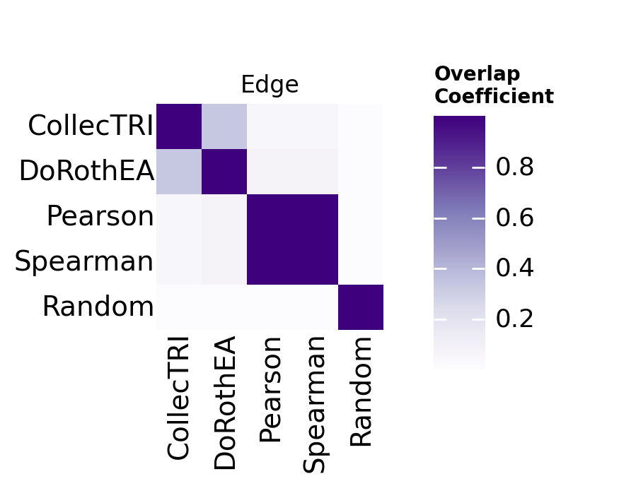
Then we can compute different statistics across a collection of GRNs. For example we can compute their similarity at the source, cre, target and edge levels:

oc_df = gt.tl.ocoeff(grn_dict)
oc_df

	grn_a	grn_b	source	cre	target	edge
0	CollecTRI	DoRothEA	0.790960	0.585267	0.578685	0.333719
1	CollecTRI	Pearson	0.706271	0.699338	0.667391	0.047101
2	CollecTRI	Spearman	0.706271	0.699338	0.667391	0.047101
3	CollecTRI	Random	0.287129	0.069757	0.149415	0.000308
4	DoRothEA	Pearson	0.672316	0.716953	0.691235	0.071561
5	DoRothEA	Spearman	0.672316	0.716953	0.691235	0.071561
6	DoRothEA	Random	0.265537	0.070636	0.143426	0.000308
7	Pearson	Spearman	1.000000	1.000000	1.000000	1.000000
8	Pearson	Random	0.415929	0.109708	0.290279	0.002157
9	Spearman	Random	0.415929	0.109708	0.290279	0.002157

We can visualize this as a matrix. Here we can see that methods tend to produce very different networks at the edge level, as measured by the overlap coefficient.

Note

We use the overlap coefficient instead of the Jaccard index because GRN methods produce networks of vastly different sizes. The overlap coefficient normalizes to the smaller network:

$$\text{Overlap}(A, B) = \frac{|A \cap B|}{\min(|A|, |B|)}$$

For example, if method A infers 1,000 edges, method B infers 10,000, and they share 900 edges:

• Jaccard = 900 / 10,100 ≈ 0.09 (suggests almost no agreement, but this is driven by the size difference)

• Overlap = 900 / 1,000 = 0.90 (90% of the smaller network’s edges are recovered)

The overlap coefficient asks the more meaningful question: to what extent is the smaller network’s regulatory logic recovered in the larger network?

gt.pl.heatmap(oc_df, level='edge', order=grn_dict.keys())

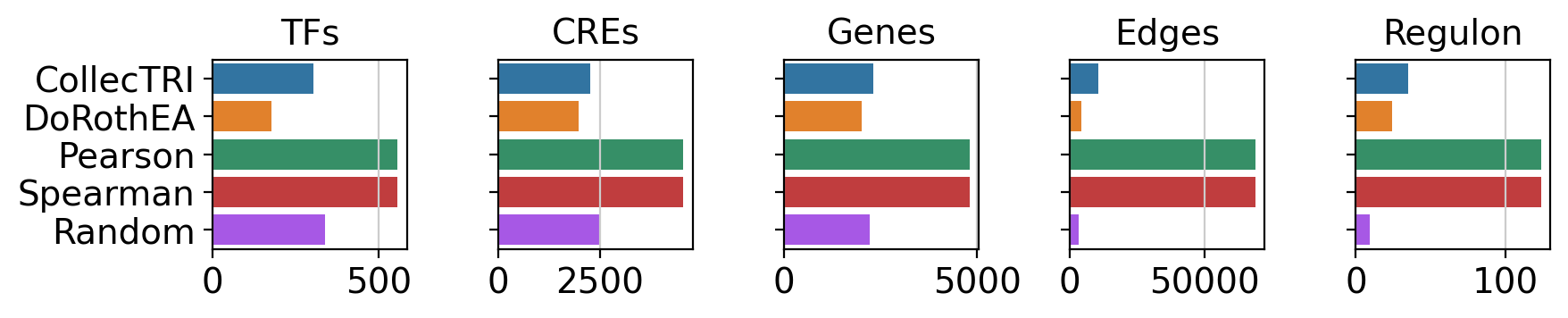
We can also compute network size statistics like:

• Number of unique sources (TFs)

• Number of unique CREs

• Number of unique target genes

• Number of edges

• Mean regulon size (how many targets does a TF have)

st_df = gt.tl.stats(grn_dict)
st_df

	name	n_sources	n_cres	n_targets	n_edges	mean_regulon_size
0	CollecTRI	303	2265	2300	10658	35.174917
1	DoRothEA	177	1982	2008	4318	24.395480
2	Pearson	558	4561	4793	68940	123.548387
3	Spearman	558	4561	4793	68940	123.548387
4	Random	339	2534	2222	3246	9.575221

Which we can also visualize. Here we see that, for example, correlation-based methods Pearson and Spearman produce GRNs that are bigger than literature-derived networks (CollecTRI and DoRothEA) or the random network.

gt.pl.stats(st_df)

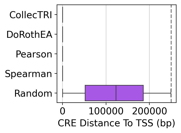
Another useful statistic to compute is the distance of CREs to the TSS of their target genes.

dt_df = gt.tl.cre_to_tss_distance(grns=grn_dict, organism='hg38')
dt_df

	grn	cre	target	distance
0	CollecTRI	chr7-87600646-87601146	ABCB1	0
1	CollecTRI	chr4-88230899-88231399	ABCG2	0
2	CollecTRI	chr17-78186409-78186909	AFMID	0
3	CollecTRI	chr7-16804717-16805217	AGR2	0
4	CollecTRI	chr5-320864-321364	AHRR	0
...	...	...	...	...
16648	Random	chr3-114291520-114292020	ZBTB20-AS5	152500
16649	Random	chr4-70688045-70688545	MOB1B	212780
16650	Random	chr6-26045025-26045525	H2BC3	313
16651	Random	chrX-112642263-112642763	AMOT	197051
16652	Random	chrX-2889156-2889656	ARSD	38682

16653 rows × 4 columns

Which we can visualize using the plot below. Here we see that only the Random network uses distal CREs; the other methods rely on proximal CREs when defining TF-CRE-Gene interactions.

gt.pl.cre_to_tss_distance(dt_df, thr_distance=250_000)

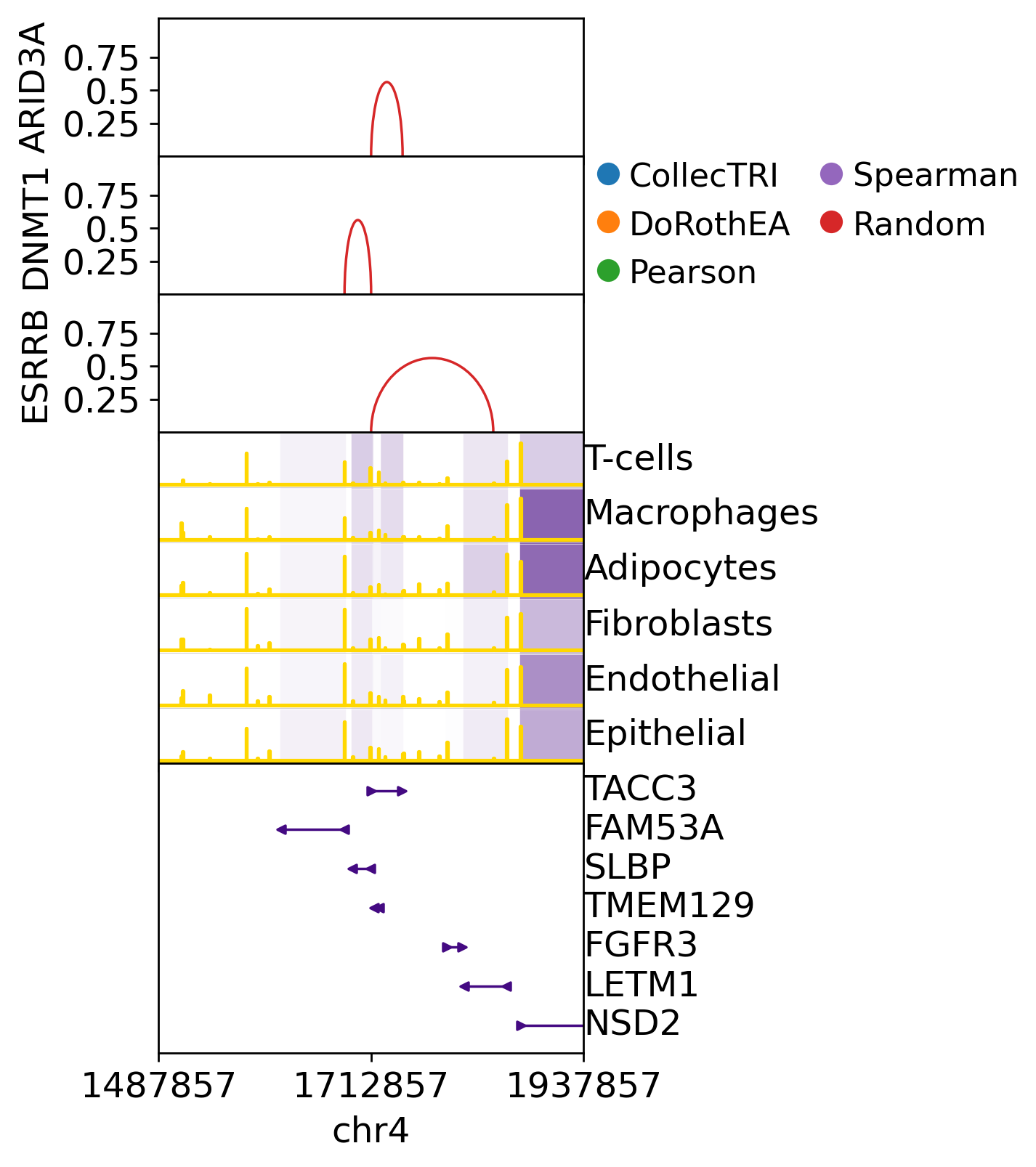
We can also plot specific TF-CRE-Gene interactions on the genome. In the below plot we see at the top the TF-CRE-Gene interaction, the height means that it has more score than other interactions in that network. In the middle we see the expression of the target gene and its neighbours (Purple), and in yellow we see the accessibility of chromatin peaks (height means more accesibility). On the bottom there is the genome annotation, where genes are.

gt.pl.links(mdata=breast, grn=grn_dict, target='TACC3', tfs=['ARID3A', 'DNMT1', 'ESRRB'], w_size=225_000)

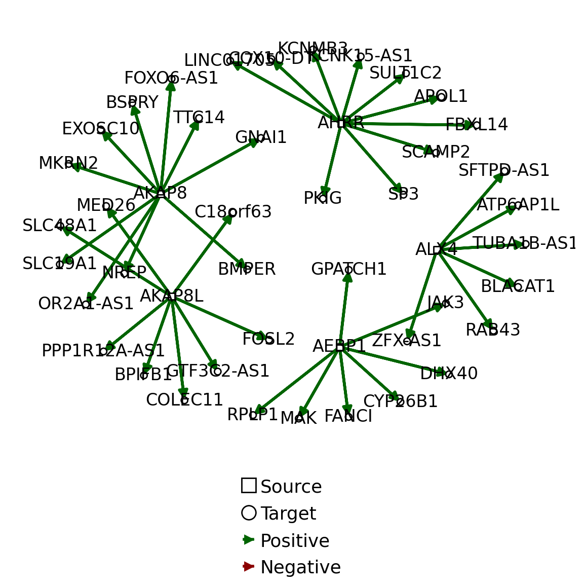
We can visualize the network also as a graph.

dc.pl.network(net=grn_dict['Random'], figsize=(6, 6))