Evaluating multimodal GRNs

Evaluating a multimodal gene regulatory network (GRN) requires two ingredients: a multiome dataset, comprising paired single-nucleus RNA-seq and ATAC-seq measurements, and a GRN inferred from that dataset. Together, these allow systematic assessment of whether the inferred regulatory relationships are supported by independent lines of evidence.

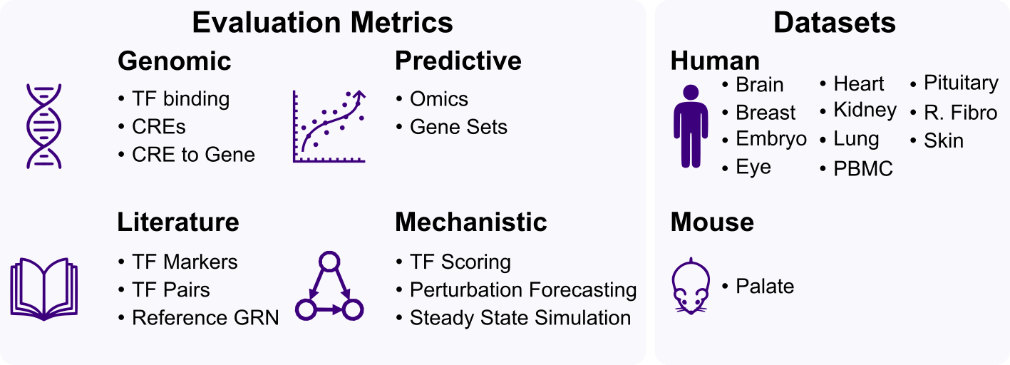
gretapy organizes evaluation into four complementary metric categories:

• Genomic: assesses whether GRN elements (TF binding sites, CREs, CRE-to-gene links) are supported by genome-wide measurements.

• Predictive: tests whether the GRN topology can predict molecular readouts, such as gene expression from TF activity or the presence of active gene sets.

• Literature: checks whether the TFs, TF-TF interactions, and TF-gene pairs in the GRN are supported by curated, experimentally validated evidence from the scientific literature.

• Mechanistic: evaluates whether the GRN can reproduce functional outcomes, including TF activity in perturbation experiments, gene expression changes after TF knockouts, and cell-type-specific steady states.

To support evaluation out of the box, gretapy provides 12 already-processed multimodal datasets spanning diverse human and mouse tissues and cell types. Each metric category can draw from multiple independent databases (e.g. ChIP-Atlas, ReMap2022, and UniBind for TF binding) or involve multiple subtasks (e.g. gene expression and chromatin accessibility prediction within the Omics metric), resulting in 25 distinct evaluation tasks across datasets. This multi-task design ensures that strong performance reflects consistency across diverse and orthogonal criteria, offering a robust and holistic view of GRN quality.

For each evaluation task, performance is quantified by defining true positives (TP), false positives (FP), and false negatives (FN) (Table 1). Precision and recall are then computed and summarized into an $F_{0.1}$ score, which weights precision ten times more than recall (β = 0.1), reflecting the principle that in GRN evaluation, predicting a small set of high-confidence edges is more informative than recovering many noisy ones.

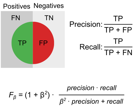
Table 1. Definition of evaluation tasks. TP: true positive; FP: false positive; FN: false negative.

Category	Task	TP	FP	FN
Genomic	TF Binding	TF-CRE in GRN and in binding collection	TF-CRE in GRN but not in collection	TF-CRE not in GRN but in collection
Genomic	CREs	CRE in GRN and in annotation	CRE in GRN but not in annotation	CRE not in GRN but in annotation
Genomic	CRE to Gene	CRE-Gene in GRN and in annotation	CRE-Gene in GRN but not in annotation	CRE-Gene not in GRN but in annotation
Predictive	Omics	Omic feature in GRN with significant predicted–observed correlation	Omic feature in GRN with insignificant correlation	Omic feature not in GRN but in dataset
Predictive	Gene Sets	Gene set in GRN and predicted present in omics data	Gene set in GRN but not in omics data	Gene set not in GRN but in omics data
Literature	TF Markers	TF in GRN and in marker collection	TF in GRN but not in collection	TF not in GRN but in collection
Literature	TF Pairs	TF-TF in GRN and in interactions collection	TF-TF in GRN but not in collection	TF-TF not in GRN but in collection
Literature	Reference GRN	TF-Gene in GRN and in reference collection	TF-Gene in GRN but not in collection	TF-Gene not in GRN but in collection
Mechanistic	TF Scoring	TF in GRN with significant activity score for perturbation	TF in GRN with insignificant activity score	TF not in GRN but in perturbation experiment
Mechanistic	Perturbation Forecasting	TF targets in GRN with significant predicted–observed correlation	TF targets in GRN with insignificant correlation	TF not in GRN but in perturbation experiment
Mechanistic	Steady State Simulation	Steady state matching one cell type	Steady state matching multiple or no cell types	Cell type not generated but present in dataset

Several evaluation tasks are made context-specific by filtering their reference databases using tissue- or cell-type-relevant terms. For example, when evaluating a dataset derived from heart tissue, only TF binding peaks annotated to cardiac cell types are retained; similarly, for brain datasets, only neuronal and glial annotations are used. This filtering ensures that evaluation reflects whether methods recover regulatory interactions relevant to the biological system under study, rather than generic genome-wide associations.

In this vignette, we begin by evaluating a toy GRN against a toy multiome dataset designed to simulate a PBMC-like tissue comprising B cells, T cells, and monocytes, with TF-gene interactions and marker genes grounded in prior biological knowledge. We walk through individual evaluation metrics step by step. We then demonstrate how to run the full benchmark across all 12 datasets and 25 tasks, and how to visualize and compare results against the precomputed scores of the 20 methods evaluated in the original GRETA manuscript.

On a single dataset

Let’s start by importing the toy dataset, which contains a multiome dataset as a MuData object, and a GRN that has been “inferred” from this data as a pandas dataframe.

Note

It is a requirement that features in the GRN, like CREs and Genes, are available as features in the multiome dataset, else it will throw an error.

import gretapy as gt
import pandas as pd

mdata, grn = gt.ds.toy()

mdata

MuData object with n_obs × n_vars = 60 × 93
  obs:	'celltype'
  2 modalities
    rna:	60 x 30
    atac:	60 x 63

grn.head()

	source	cre	target	score
0	PAX5	chr16-28926950-28927450	CD19	0.85
1	PAX5	chr16-28936000-28936500	CD19	0.72
2	PAX5	chr11-60443809-60444309	MS4A1	0.78
3	PAX5	chr19-41827233-41827733	CD79A	0.72
4	PAX5	chr18-63073346-63073846	BCL2	0.68

For this vignette, we use the toy dataset to keep computations fast. In practice, gretapy provides 12 pre-processed multiome datasets spanning diverse human and mouse tissues and cell types, which can be listed with gt.show_datasets().

gt.show_datasets()

	organism	name	pubmed	geo
0	hg38	Brain	38491288	GSE193688
1	hg38	Breast	39122969	None
2	hg38	Embryo	37369347	GSE218314
3	hg38	Eye	36277849	GSE196235
4	hg38	Heart	37438528	None
5	hg38	Kidney	37333123	None
6	hg38	Lung	39266564	GSE241468
7	hg38	PBMC	None	None
8	hg38	Pituitary	35263594	GSE178454
9	hg38	Repr. Fibroblasts	37873116	GSE242419
10	hg38	Skin	36121124	GSE207335
11	mm10	Palate	38280850	GSE218576

These can then be easily downloaded with gt.ds.read_dts, for example:

mdata = gt.ds.read_dts(organism='hg38', dts_name='PBMC')

Note

Any data gretapy downloads, it will be available at ./gretapy_data

Next, we check which metrics are available for the given organism:

metrics = gt.show_metrics(organism='hg38')
metrics

	category	metric	db
0	Genomic	CRE to Gene	eQTL Catalogue
1	Genomic	CREs	ENCODE Blacklist
2	Genomic	CREs	ENCODE CREs
3	Genomic	CREs	GWAS Catalog
4	Genomic	CREs	Promoters
5	Genomic	CREs	Zhang21
6	Genomic	CREs	phastCons
7	Genomic	TF Binding	ChIP-Atlas
8	Genomic	TF Binding	ReMap 2022
9	Genomic	TF Binding	UniBind
10	Literature	Reference GRN	CollecTRI
11	Literature	TF Markers	HPA
12	Literature	TF Markers	TF-Marker
13	Literature	TF Pairs	Europe PMC
14	Literature	TF Pairs	IntAct
15	Mechanistic	Perturbation Forecasting	KnockTF (forecasting)
16	Mechanistic	Steady State Simulation	Boolean rules
17	Mechanistic	TF Scoring	KnockTF (scoring)
18	Predictive	Gene Sets	Hallmarks
19	Predictive	Gene Sets	KEGG
20	Predictive	Gene Sets	PROGENy
21	Predictive	Gene Sets	Reactome
22	Predictive	Omics	CRE ~ TFs
23	Predictive	Omics	Gene ~ CREs
24	Predictive	Omics	Gene ~ TFs

As mentioned in the introduction, some metrics filter their reference databases using tissue- or cell-type-relevant terms to ensure context-specific evaluation. Since our toy dataset simulates a PBMC-like tissue, we reuse the terms associated with the PBMC dataset. These terms are passed to gt.tl.eval_grn_dataset and used to restrict, for example, TF binding peaks to those annotated in relevant blood cell types.

Note

When working with a custom multiome dataset not available in gretapy you will need to define which terms to filter for. You can check the full list of terms across evaluation databases by running:

gt.show_terms(organism='hg38')

Here’s how to retrieve them:

terms = gt.get_terms('PBMC')

To evaluate a GRN against a dataset, use the gt.tl.eval_grn_dataset function. The metrics argument controls which metrics to run: you can pass a specific database or subtask name (e.g. TF-Marker), a metric name (e.g. TF Markers), or a metric category (e.g. Literature). If set to None, all available metrics are run. Below is an example evaluating the TF-Marker database from the TF Markers task in the Literature category:

df = gt.tl.eval_grn_dataset(
    organism='hg38',
    grn=grn,
    dataset=mdata,
    terms=terms,
    metrics='TF-Marker'
)
df

	class	task	db	precision	recall	f01
0	Literature	TF Markers	TF-Marker	0.666667	0.444444	0.663383

The output reports the category, task, database or subtask name, along with precision, recall, and $F_{0.1}$ score. Let’s try another example, the ChIP-Atlas database from the TF Binding task within the Genomic category:

df = gt.tl.eval_grn_dataset(
    organism='hg38',
    grn=grn,
    dataset=mdata,
    terms=terms,
    metrics='ChIP-Atlas'
)
df

	class	task	db	precision	recall	f01
0	Genomic	TF Binding	ChIP-Atlas	0.057692	0.038961	0.057419

Of course, we can also run multiple databases or metrics in a single call. Here we repeat the same two evaluations together:

df = gt.tl.eval_grn_dataset(
    organism='hg38',
    grn=grn,
    dataset=mdata,
    terms=terms,
    metrics=['TF-Marker', 'ChIP-Atlas']
)
df

	class	task	db	precision	recall	f01
0	Genomic	TF Binding	ChIP-Atlas	0.057692	0.038961	0.057419
1	Literature	TF Markers	TF-Marker	0.666667	0.444444	0.663383

On multiple datasets

To run the evaluation across multiple datasets and metrics, one could loop the gt.tl.eval_grn_dataset function, or use the gt.tl.benchmark function directly instead.

This function accepts as input a dictionary of GRNs called grns. It’s format should be:

grn_dict = {
  "MethodA": {
    "hg38": {
      "PBMC": pd.DataFrame,
      ...
    }
  }
}

For each method, for each organism, for each dataset have a GRN as a pandas dataframe. Then simply run:

df = gt.tl.benchmark(grns=grn_dict)

Note

This line can take from 1 to 2 hours to run depending on your internet connection and number of CPUs available.

It will also download 40 GB total space of datasets and evaluation databases, so make sure you have enough space on disk.

If you have a custom GRN inference method that you would like to benchmark across all gretapy datasets, here’s the logic you should follow:

import gretapy as gt

# Get available datasets
lst_dts = gt.show_datasets()[['organism', 'name']].values

for org, dts in lst_dts:
    # Retrieve individual dataset
    mdata = gt.ds.read_dts(organism=org, dts_name=dts, verbose=True)
    # Run custom GRN method
    grn = ...  # use mdata as input
    # Save
    grn_dict['CollecTRI'][org][dts] = grn

# Run benchmark
mth_res = gt.tl.benchmark(grns=grn_dict)

Once it runs it should look like this example result for an imaginary method:

mth_res = gt.ds.read_imaginary_metrics()
mth_res

	class	task	db	organism	dataset	name	precision	recall	f01
0	Predictive	Gene Sets	Hallmarks	hg38	Eye	ImaginaryMethod	0.200000	0.250000	0.200397
1	Predictive	Gene Sets	Hallmarks	hg38	Kidney	ImaginaryMethod	0.181818	0.800000	0.183220
2	Predictive	Gene Sets	Hallmarks	hg38	Breast	ImaginaryMethod	0.217391	0.909091	0.219041
3	Predictive	Gene Sets	Hallmarks	hg38	Skin	ImaginaryMethod	0.571429	0.320000	0.567018
4	Predictive	Gene Sets	Hallmarks	hg38	Brain	ImaginaryMethod	0.071429	0.500000	0.072040
...	...	...	...	...	...	...	...	...	...
286	Literature	TF Pairs	Europe PMC	hg38	Embryo	ImaginaryMethod	0.014936	0.173477	0.015073
287	Literature	TF Pairs	Europe PMC	hg38	Heart	ImaginaryMethod	0.056566	0.058639	0.056585
288	Literature	TF Pairs	Europe PMC	hg38	PBMC	ImaginaryMethod	0.057269	0.016414	0.055891
289	Literature	TF Pairs	Europe PMC	hg38	Pituitary	ImaginaryMethod	0.127566	0.182965	0.127950
290	Literature	TF Pairs	Europe PMC	hg38	Lung	ImaginaryMethod	0.259259	0.014768	0.222747

291 rows × 9 columns

We can then concatenate the results from our imaginary method with the original results from the gretapy manuscript.

old_res = gt.ds.read_metrics()
old_res

	class	task	db	organism	dataset	name	precision	recall	f01
0	Predictive	Gene Sets	Hallmarks	hg38	Eye	CellOracle	0.500000	0.750000	0.501656
1	Predictive	Gene Sets	Hallmarks	hg38	Eye	CollecTRI	0.080000	1.000000	0.080735
2	Predictive	Gene Sets	Hallmarks	hg38	Eye	CREMA	0.181818	0.500000	0.182971
3	Predictive	Gene Sets	Hallmarks	hg38	Eye	Dictys	0.187500	0.750000	0.188903
4	Predictive	Gene Sets	Hallmarks	hg38	Eye	DIRECT-NET	0.111111	0.500000	0.111973
...	...	...	...	...	...	...	...	...	...
5565	Literature	TF Pairs	Europe PMC	hg38	Lung	SCENIC	0.119403	0.008439	0.105649
5566	Literature	TF Pairs	Europe PMC	hg38	Lung	SCENIC+	0.061911	0.048523	0.061743
5567	Literature	TF Pairs	Europe PMC	hg38	Lung	scGPT	0.043919	0.013713	0.042982
5568	Literature	TF Pairs	Europe PMC	hg38	Lung	scMTNI	0.000000	0.000000	0.000000
5569	Literature	TF Pairs	Europe PMC	hg38	Lung	Spearman	0.014317	0.210970	0.014451

5570 rows × 9 columns

res = pd.concat([mth_res, old_res])
res

	class	task	db	organism	dataset	name	precision	recall	f01
0	Predictive	Gene Sets	Hallmarks	hg38	Eye	ImaginaryMethod	0.200000	0.250000	0.200397
1	Predictive	Gene Sets	Hallmarks	hg38	Kidney	ImaginaryMethod	0.181818	0.800000	0.183220
2	Predictive	Gene Sets	Hallmarks	hg38	Breast	ImaginaryMethod	0.217391	0.909091	0.219041
3	Predictive	Gene Sets	Hallmarks	hg38	Skin	ImaginaryMethod	0.571429	0.320000	0.567018
4	Predictive	Gene Sets	Hallmarks	hg38	Brain	ImaginaryMethod	0.071429	0.500000	0.072040
...	...	...	...	...	...	...	...	...	...
5565	Literature	TF Pairs	Europe PMC	hg38	Lung	SCENIC	0.119403	0.008439	0.105649
5566	Literature	TF Pairs	Europe PMC	hg38	Lung	SCENIC+	0.061911	0.048523	0.061743
5567	Literature	TF Pairs	Europe PMC	hg38	Lung	scGPT	0.043919	0.013713	0.042982
5568	Literature	TF Pairs	Europe PMC	hg38	Lung	scMTNI	0.000000	0.000000	0.000000
5569	Literature	TF Pairs	Europe PMC	hg38	Lung	Spearman	0.014317	0.210970	0.014451

5861 rows × 9 columns

We can then visualize the updated results in the summary heatmap plot at the metric class level:

gt.pl.ranking(res, level='class', figsize=(5, 5))

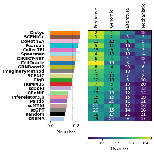
This heatmap color indicates mean $F_{0.1}$ scores, and the numbers indicate the ranking inside each metric class (lower is better).

Alternatively, we can visualize the results at finer resolution, grouped by individual evaluation task, to see which specific databases or subtasks drive the differences between methods:

gt.pl.ranking(res, level='task')

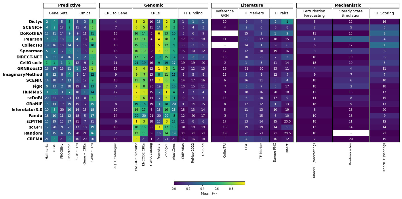
In this case, ImaginaryMethod does not manage to outperform the top-performing methods in the benchmark. To understand where a method falls short, inspecting the task-level plot can help identify which metric categories drive its ranking.